`bayesmsm` for longitudinal data with informative right-censoring

Introduction

The bayesmsm package enables easy implementation of the Bayesian marginal structural models (BMSMs) for longitudinal data. The methodology of BMSMs can be divided into 2 estimation steps:
- Step 1. Bayesian treatment effect weight estimation
- Step 2. Bayesian non-parametric bootstrap to maximize the utility function with respect to the causal effect
For Step 1, we estimate treatment weights $w_{ij}$ using posterior samples of the $\alpha$ and $\beta$ via fitting a series of logistic regressions in a Bayesian framework. The package is able to handle longitudinal data without and with right-censoring. For Step 2, $P_n(v_{ij})$ is estimated via non-parametric Bayesian bootstrap with $Dir(1,...,1)$ sampling weights.
The main functions in this package include:
- bayesweight: Calculates Bayesian weights for subject-specific treatment effects.
- bayesweight_cen: Calculates Bayesian weights for subject-specific treatment effects with right-censored data.
- bayesmsm: Estimates marginal structural models using the calculated Bayesian weights.
- plot_ATE: Plots the estimated Average Treatment Effect (ATE).
- plot_APO: Plots the estimated Average Potential Outcome (APO).
- plot_est_box: Plots the distribution of estimated treatment effects.
- summary_bayesmsm: Summarizes the model results from bayesmsm.
Installation
- To install the bayesmsm package, you can use the devtools package to install it directly from GitHub.

Simulated observational data with right-censoring

We illustrate the implementation of the bayesmsm package using a simulated dataset. The simulated dataset contains right-censoring with a binary end-of-study outcome. This example will provide a comprehensive understanding of how to apply the package to real-world data.

Dataset Introduction

In this simulation study, we use a simulated longitudinal dataset to mimic complex real-world clinical data with right-censoring. This dataset consists of 500 patients observed over 3 visits. The binary outcome variable represents the end-of-study status of the patients. The dataset includes baseline covariates $L11$ and $L21$ , with $L11$ being binary and $L21$ continuous. Time-dependent covariates $L12$ and $L22$ are observed at the second visit, and $L13$ and $L23$ at the third visit. The treatment variables are represented as $A1$ , $A2$ , and $A3$ for the three visits. Right-censoring indicators are represented as $C1$ , $C2$ , and $C3$ . For example, for observations with $C1 = 1$ , all records at or after visit 1 were censored.

Description of Simulated Right-Censored Dataset
Variable	Description
L11	Baseline covariate (binary)
L21	Baseline covariate (continuous)
A1, A2, A3	Treatment assignments (binary)
C1, C2, C3	Right-censoring indicators
Y	End-of-study outcome (binary)

# example simulated causal data with censoring;
simdat_cen <- read.csv(system.file("extdata", "sim_causal.csv", package = "bayesmsm"))

# look at the data;
head(simdat_cen)
#>   L11         L21 A1 L12        L22 A2 L13        L23 A3 C1 C2 C3  Y
#> 1   0 -0.37560287 NA  NA         NA NA  NA         NA NA  1 NA NA NA
#> 2   1 -0.56187636 NA  NA         NA NA  NA         NA NA  1 NA NA NA
#> 3   0 -0.34391723  1   1 -0.8053290  1   1 -2.5508298  1  0  0  0  0
#> 4   1  0.09049665  1   1 -1.7754302  1   1 -2.2849997  0  0  0  0  0
#> 5   1  1.59850877  1   1  0.5604468  1   0  2.1787137  0  0  0  0  1
#> 6   0 -0.08856511  0   0  1.4798603  0   1  0.7025151  0  0  0  0  1

Bayesian treatment effect weight estimation using `bayesweight_cen`

Next, we use the bayesweight_cen function to estimate the weights with censoring. We specify the treatment and censoring models for each time point, including the relevant covariates.

Parameters Description:
- trtmodel.list: A list of formulas corresponding to each time point with the time-specific treatment variable on the left hand side and pre-treatment covariates to be balanced on the right hand side. Interactions and functions of covariates are allowed.
- cenmodel.list: A list of formulas of the censoring model with the censoring indicators on the left hand side and the covariates prior to the censoring indicators on the right hand side.
- data: The dataset containing all the variables specified in trtmodel.list.
- n.chains: Number of MCMC chains to run. For non-parallel execution, this should be set to 1. For parallel execution, it requires at least 2 chains.
- n.iter: Total number of iterations for each chain (including burn-in).
- n.burnin: Number of iterations to discard at the beginning of the simulation (burn-in).
- n.thin: Thinning rate for the MCMC sampler.
- seed: Seed to ensure reproducibility.
- parallel: Logical flag indicating whether to run the MCMC chains in parallel. Default is TRUE.

weights_cen <- bayesweight_cen(trtmodel.list = list(A1 ~ L11 + L21,
                                                A2 ~ L11 + L21 + L12 + L22 + A1,
                                                A3 ~ L11 + L21 + L12 + L22 + A1 + L13 + L23 + A2),
                           cenmodel.list = list(C1 ~ L11 + L21,
                                                C2 ~ L11 + L21 + A1,
                                                C3 ~ L11 + L21 + A1 + L12 + L22 + A2),
                           data = simdat_cen,
                           n.chains = 1,
                           n.iter = 200,
                           n.burnin = 100,
                           n.thin = 1,
                           seed = 890123,
                           parallel = FALSE)
#> Compiling model graph
#>    Resolving undeclared variables
#>    Allocating nodes
#> Graph information:
#>    Observed stochastic nodes: 4836
#>    Unobserved stochastic nodes: 44
#>    Total graph size: 16501
#> 
#> Initializing model
summary(weights_cen$weights)
#>    Min. 1st Qu.  Median    Mean 3rd Qu.    Max.    NA's 
#>  0.3966  1.0348  1.7860  2.7652  3.5724 21.8808     136

Similarly, the function will automatically run MCMC with JAGS based on the specified treatment and censoring model inputs, generating a JAGS model string as part of the function output. The function returns a list containing the updated weights for subject-specific treatment and censoring effects as well as the JAGS model.

We can print and view the JAGS model stored in model_string from the above function output:

cat(weights_cen$model_string)
#> model{
#> 
#> for (i in 1:N1) {
#> 
#> # conditional model;
#> A1[i] ~ dbern(p1[i])
#> logit(p1[i]) <- b10 + b11*L11[i] + b12*L21[i]
#> C1[i] ~ dbern(cp1[i])
#> logit(cp1[i]) <- s10 + s11*L11[i] + s12*L21[i]
#> 
#> # marginal model;
#> A1s[i] ~ dbern(p1s[i])
#> logit(p1s[i]) <- bs10
#> C1s[i] ~ dbern(cp1s[i])
#> logit(cp1s[i]) <- ts10
#> }
#> 
#> for (i in 1:N2) {
#> 
#> # conditional model;
#> A2[i] ~ dbern(p2[i])
#> logit(p2[i]) <- b20 + b21*L11[i] + b22*L21[i] + b23*L12[i] + b24*L22[i] + b25*A1[i]
#> C2[i] ~ dbern(cp2[i])
#> logit(cp2[i]) <- s20 + s21*L11[i] + s22*L21[i] + s23*A1[i]
#> 
#> # marginal model;
#> A2s[i] ~ dbern(p2s[i])
#> logit(p2s[i]) <- bs20 + bs21*A1s[i]
#> C2s[i] ~ dbern(cp2s[i])
#> logit(cp2s[i]) <- ts20 + ts21*A1s[i]
#> }
#> 
#> for (i in 1:N3) {
#> 
#> # conditional model;
#> A3[i] ~ dbern(p3[i])
#> logit(p3[i]) <- b30 + b31*L11[i] + b32*L21[i] + b33*L12[i] + b34*L22[i] + b35*A1[i] + b36*L13[i] + b37*L23[i] + b38*A2[i]
#> C3[i] ~ dbern(cp3[i])
#> logit(cp3[i]) <- s30 + s31*L11[i] + s32*L21[i] + s33*A1[i] + s34*L12[i] + s35*L22[i] + s36*A2[i]
#> 
#> # marginal model;
#> A3s[i] ~ dbern(p3s[i])
#> logit(p3s[i]) <- bs30 + bs31*A1s[i] + bs32*A2s[i]
#> C3s[i] ~ dbern(cp3s[i])
#> logit(cp3s[i]) <- ts30 + ts31*A1s[i] + ts32*A2s[i]
#> }
#> 
#> # Priors
#> b10 ~ dunif(-10, 10)
#> b11 ~ dunif(-10, 10)
#> b12 ~ dunif(-10, 10)
#> s10 ~ dunif(-10, 10)
#> s11 ~ dunif(-10, 10)
#> s12 ~ dunif(-10, 10)
#> bs10 ~ dunif(-10, 10)
#> ts10 ~ dunif(-10, 10)
#> b20 ~ dunif(-10, 10)
#> b21 ~ dunif(-10, 10)
#> b22 ~ dunif(-10, 10)
#> b23 ~ dunif(-10, 10)
#> b24 ~ dunif(-10, 10)
#> b25 ~ dunif(-10, 10)
#> s20 ~ dunif(-10, 10)
#> s21 ~ dunif(-10, 10)
#> s22 ~ dunif(-10, 10)
#> s23 ~ dunif(-10, 10)
#> bs20 ~ dunif(-10, 10)
#> bs21 ~ dunif(-10, 10)
#> ts20 ~ dunif(-10, 10)
#> ts21 ~ dunif(-10, 10)
#> b30 ~ dunif(-10, 10)
#> b31 ~ dunif(-10, 10)
#> b32 ~ dunif(-10, 10)
#> b33 ~ dunif(-10, 10)
#> b34 ~ dunif(-10, 10)
#> b35 ~ dunif(-10, 10)
#> b36 ~ dunif(-10, 10)
#> b37 ~ dunif(-10, 10)
#> b38 ~ dunif(-10, 10)
#> s30 ~ dunif(-10, 10)
#> s31 ~ dunif(-10, 10)
#> s32 ~ dunif(-10, 10)
#> s33 ~ dunif(-10, 10)
#> s34 ~ dunif(-10, 10)
#> s35 ~ dunif(-10, 10)
#> s36 ~ dunif(-10, 10)
#> bs30 ~ dunif(-10, 10)
#> bs31 ~ dunif(-10, 10)
#> bs32 ~ dunif(-10, 10)
#> ts30 ~ dunif(-10, 10)
#> ts31 ~ dunif(-10, 10)
#> ts32 ~ dunif(-10, 10)
#> }

Bayesian non-parametric bootstrap to maximize the utility function with respect to the causal effect using `bayesmsm`

Using the weights estimated by bayesweight_cen, we now fit the Bayesian Marginal Structural Model and estimate the marginal treatment effects using the bayesmsm function as before. We specify the outcome model and other relevant parameters.

Parameters Description:
- ymodel: A formula representing the outcome model, which can include interactions and functions of covariates.
- nvisit: Specifies the number of visits or time points considered in the model.
- reference: The baseline or reference intervention across all visits, typically represented by a vector of zeros indicating no treatment (default is a vector of all zeros).
- comparator: The comparison intervention across all visits, typically represented by a vector of ones indicating full treatment (default is a vector of all ones).
- treatment_effect_type: A character string specifying the type of treatment effect to estimate. Options are “sq” for sequential treatment effects, which estimates effects for specific treatment sequences across visits, and “cum” for cumulative treatment effects, which assumes a single cumulative treatment variable representing the total exposure. The default is “sq”.
- family: Specifies the outcome distribution family; use “gaussian” for continuous outcomes or “binomial” for binary outcomes (default is “gaussian”).
- data: The dataset containing all variables required for the model.
- wmean: A vector of treatment assignment weights. Default is a vector of ones, implying equal weighting.
- nboot: The number of bootstrap iterations to perform for estimating the uncertainty around the causal estimates.
- optim_method: The optimization method used to find the best parameters in the model (default is ‘BFGS’).
- seed: A seed value to ensure reproducibility of results.
- parallel: A logical flag indicating whether to perform computations in parallel (default is TRUE).
- ncore: The number of cores to use for parallel computation (default is 4).

# Remove all NAs (censored observations) from the original dataset and weights
simdat_cen <- na.omit(simdat_cen)
weights_cen$weights <- na.omit(weights_cen$weights)

model <- bayesmsm(ymodel = Y ~ A1+A2+A3,
                  nvisit = 3,
                  reference = c(rep(0, 3)),
                  comparator = c(rep(1, 3)),
                  family = "binomial",
                  data = simdat_cen,
                  wmean = weights_cen$weights,
                  nboot = 50,
                  optim_method = "BFGS",
                  parallel = TRUE,
                  seed = 890123,
                  ncore = 2)
str(model)
#> List of 12
#>  $ RD_mean    : num 0.23
#>  $ RR_mean    : num 1.56
#>  $ OR_mean    : num 2.97
#>  $ RD_sd      : num 0.114
#>  $ RR_sd      : num 0.354
#>  $ OR_sd      : num 1.42
#>  $ RD_quantile: Named num [1:2] 0.0139 0.42
#>   ..- attr(*, "names")= chr [1:2] "2.5%" "97.5%"
#>  $ RR_quantile: Named num [1:2] 1.02 2.35
#>   ..- attr(*, "names")= chr [1:2] "2.5%" "97.5%"
#>  $ OR_quantile: Named num [1:2] 1.06 6.13
#>   ..- attr(*, "names")= chr [1:2] "2.5%" "97.5%"
#>  $ bootdata   :'data.frame': 50 obs. of  5 variables:
#>   ..$ effect_reference : num [1:50] 0.4624 -0.2683 -0.0994 -0.4618 -0.4679 ...
#>   ..$ effect_comparator: num [1:50] 0.629 0.938 0.901 1.018 1.142 ...
#>   ..$ RD               : num [1:50] 0.0388 0.2854 0.2359 0.348 0.373 ...
#>   ..$ RR               : num [1:50] 1.06 1.66 1.5 1.9 1.97 ...
#>   ..$ OR               : num [1:50] 1.18 3.34 2.72 4.39 5 ...
#>  $ reference  : num [1:3] 0 0 0
#>  $ comparator : num [1:3] 1 1 1

The bayesmsm function returns a model object containing the following: the mean, standard deviation, and 95% credible interval of the Risk Difference (RD), Risk Ratio (RR), and Odds Ratio (OR). It also includes a data frame containing the bootstrap samples for the reference effect, comparator effect, RD, RR, and OR, as well as the reference and comparator levels chosen by the user.

Summary function to generate result table from bayesmsm
- The summary_bayesmsm function automatically generates a summary table of the model output from the function bayesmsm.

summary_bayesmsm(model)
#>                  mean        sd        2.5%     97.5%
#> Reference  -0.1760620 0.3274180 -0.75963321 0.4380595
#> Comparator  0.7985806 0.2456904  0.36512879 1.1501634
#> RD          0.2301848 0.1136792  0.01389312 0.4199952
#> RR          1.5600476 0.3538751  1.02301493 2.3475914
#> OR          2.9669176 1.4221489  1.06257769 6.1301699

Visualization functions: `plot_ATE`, `plot_APO`, `plot_est_box`

Similarly, we can use the built-in functions as well as summary_bayesmsm to visualize and summarize the results.

Plotting the Average Treatment Effect (ATE)
- The plot_ATE function generates a plot of the estimated ATE with its 95% credible interval.

plot_ATE(model)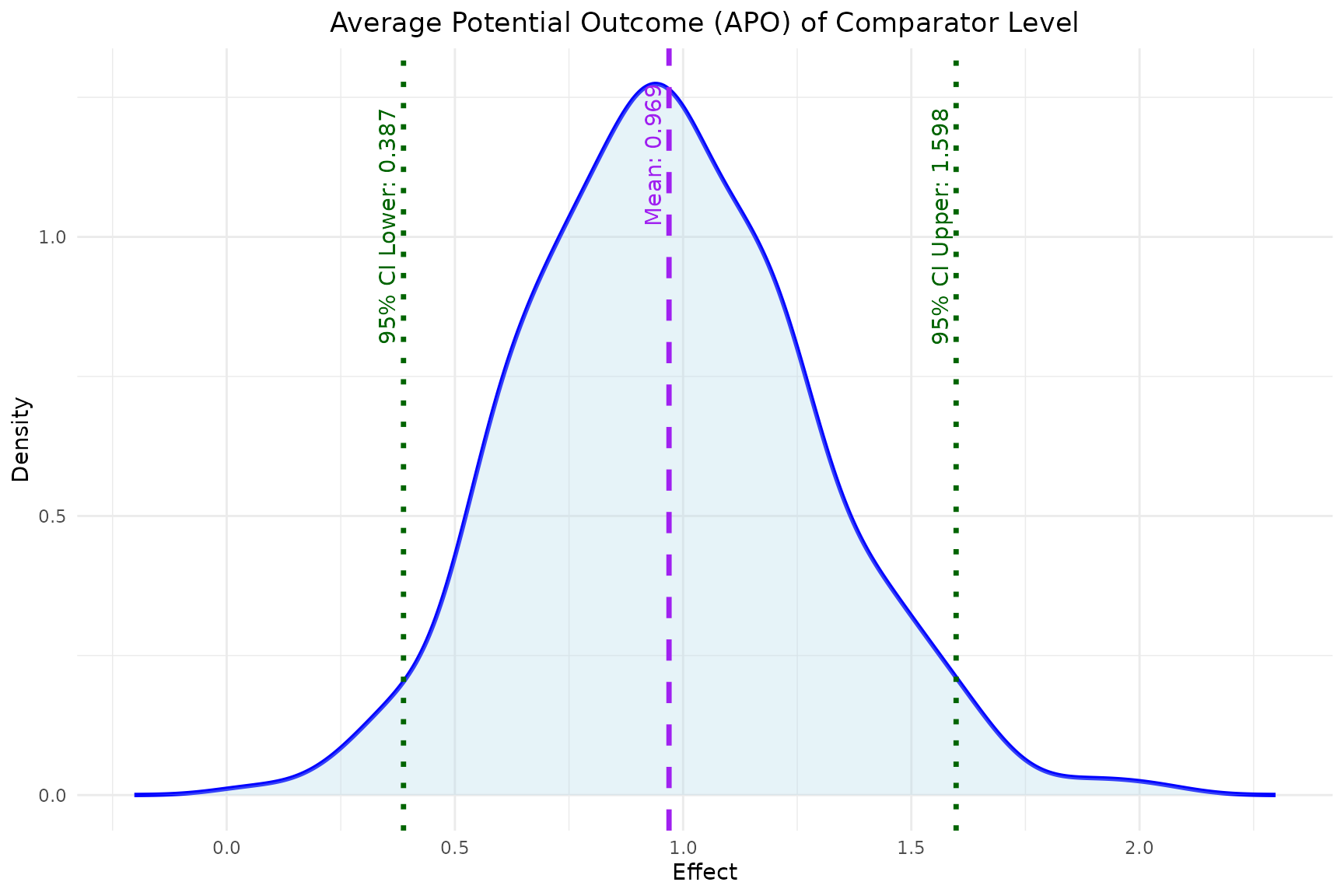

Plotting the Average Potential Outcome (APO)
- The plot_APO function plots the estimated APO for both the reference and comparator level effects.

plot_APO(model, effect_type = "effect_comparator")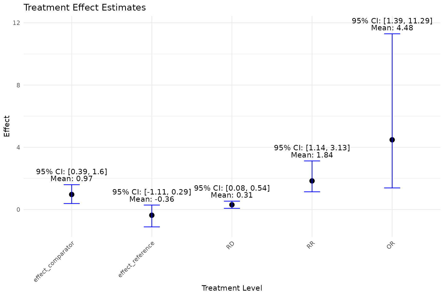

plot_APO(model, effect_type = "effect_reference")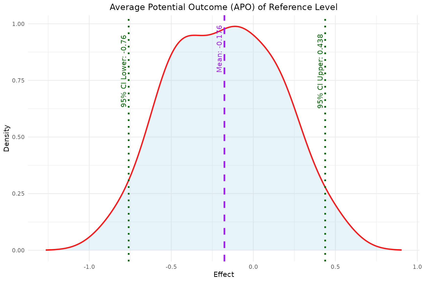

Plotting the Distribution of Estimated Treatment Effects
- The plot_est_box function generates an error bar plot of the estimated treatment effects (APO and ATE) from the bootstrap samples.

plot_est_box(model)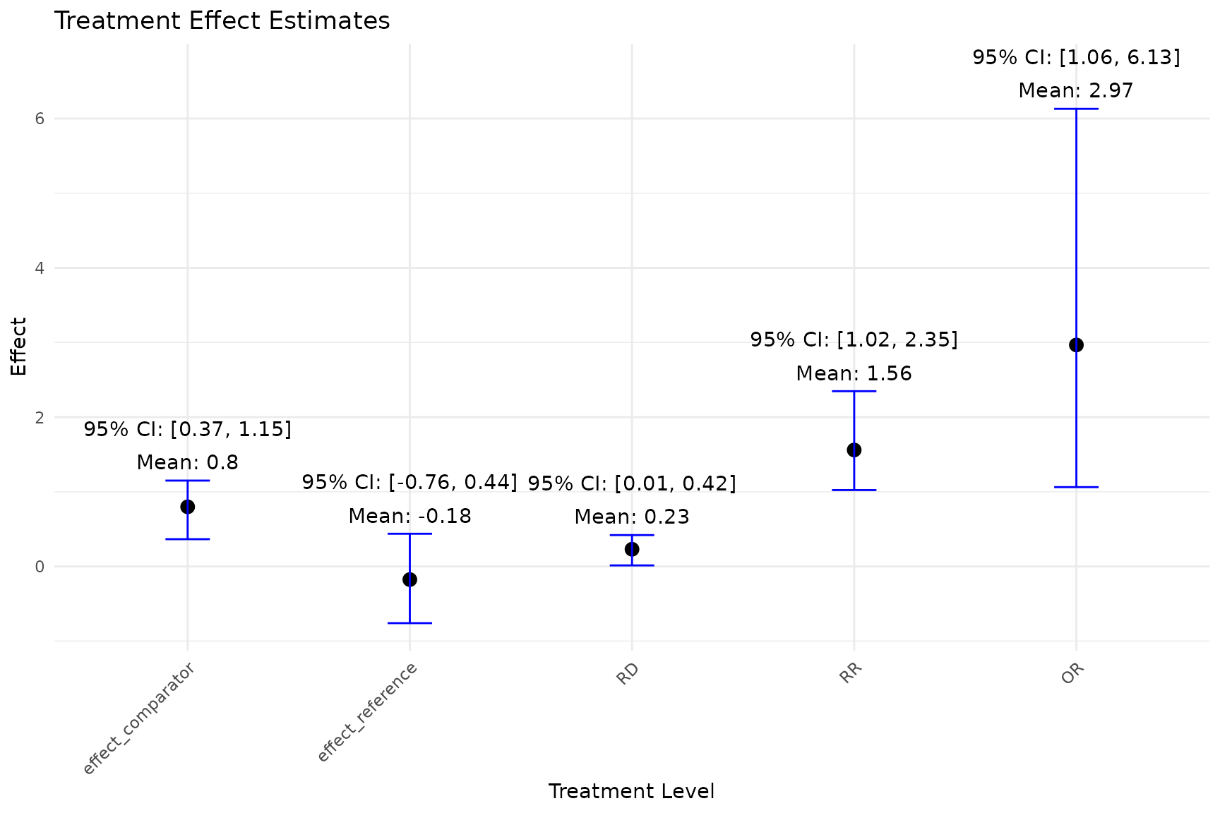

Reference

Saarela, O., Stephens, D. A., Moodie, E. E. M., & Klein, M. B. (2015). On Bayesian estimation of marginal structural models. Biometrics, 71(2), 279–288. https://doi.org/10.1111/biom.12269
Robins, J. M., Hernán, M. A., & Brumback, B. (2000). Marginal structural models and causal inference in epidemiology. Epidemiology, 11(5), 550–560. https://doi.org/10.1097/00001648-200009000-00011
Liu, K., Saarela, O., Feldman, B. M., & Pullenayegum, E. (2020). Estimation of causal effects with repeatedly measured outcomes in a Bayesian framework. Statistical Methods in Medical Research, 29(9), 2507–2519. https://doi.org/10.1177/0962280219900362

Xiao Yan, Kuan Liu